Statistics

import pandas as pd
import seaborn as sns

import statsmodels.api as sm
import statsmodels.formula.api as smf

import numpy as np
from numpy.random import default_rng

from scipy import stats

df = sm.datasets.get_rdataset("mtcars", "datasets", cache = True).data

Summary Stats

# get the data as a vector
v = df.mpg

np.mean(v)
# (https://docs.scipy.org/doc/scipy/reference/generated/scipy.stats.mode.html)
stats.mode(v, keepdims = False)
np.median(v)
np.var(v)

35.188974609374995

Simulating Data

After trying a few things, it looks like numpy is king here.

Create an RNG Object

To get started, create an RNG object that will make sure everything is initialized correctly.

rng = default_rng()

We can now go through a list of common distributions, simulate from them, and visualize to make sure we’re on the right track.

Normal/Guassian

n = 1000

# because calling the mean and sd the "mean" and "sd" would be too obvious
v_norm = rng.normal(loc = 5, scale = 2.5, size = n)
sns.kdeplot(v_norm)

<AxesSubplot: ylabel='Density'>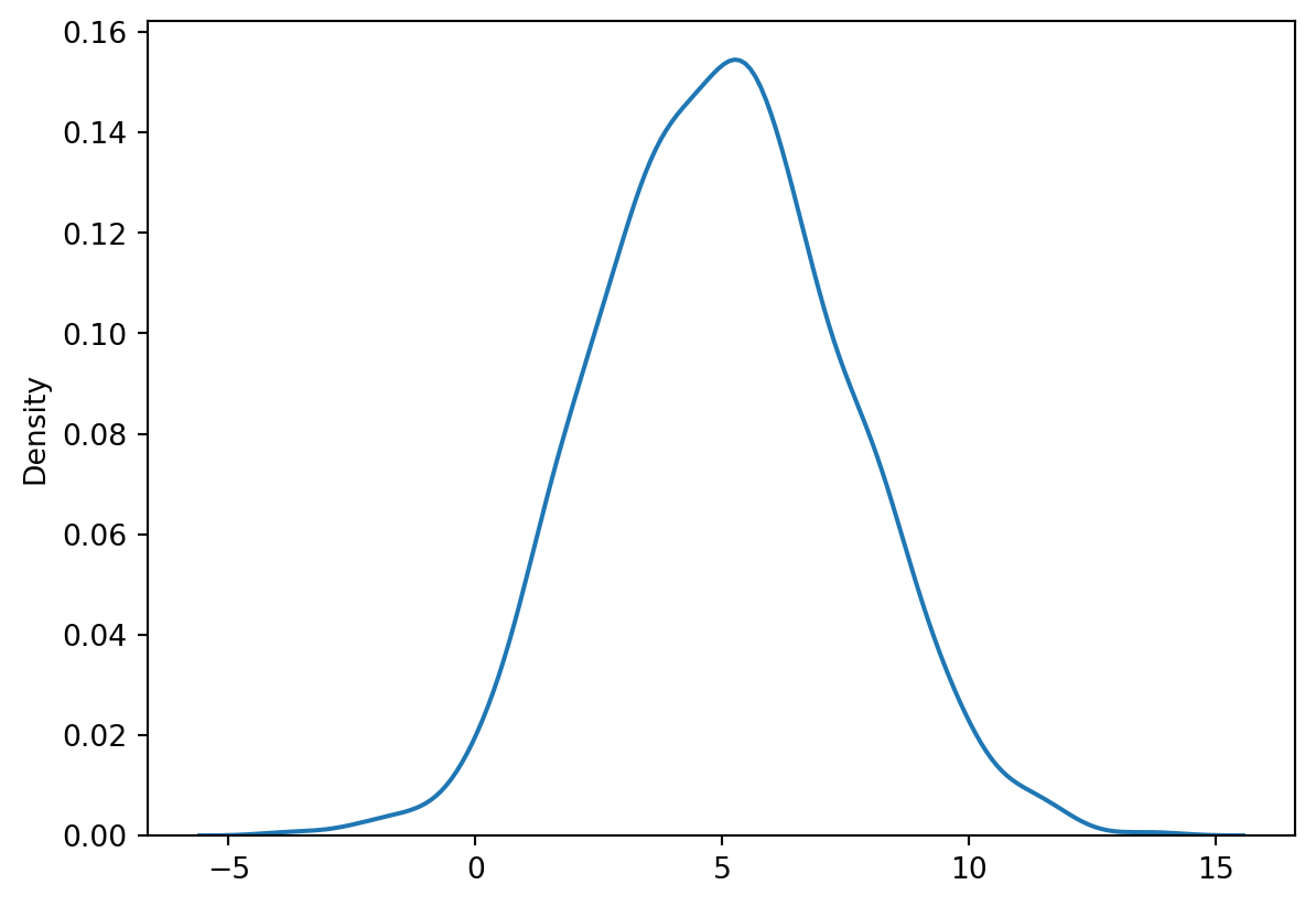

Uniform

# this makes sense lol
v_unif = rng.uniform(low = 0, high = 1, size = n)
sns.kdeplot(v_unif)

<AxesSubplot: ylabel='Density'>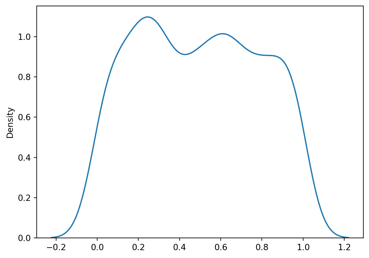

Poisson

# lamda was too long I guess
v_poisson = rng.poisson(lam = 1, size = n)
sns.histplot(v_poisson)

<AxesSubplot: ylabel='Count'>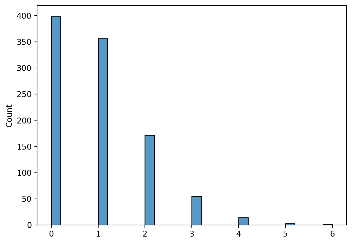

Bernoulli

# bernoulli 
# https://stackoverflow.com/questions/47012474/bernoulli-random-number-generator
v_bernoulli = rng.binomial(n = 1, p = 0.5, size = n)
sns.histplot(v_bernoulli)

<AxesSubplot: ylabel='Count'>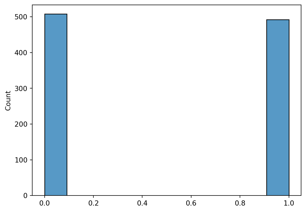

Binomial

# binomial
v_binomial = rng.binomial(n = 4, p = 0.15, size = n)
sns.histplot(v_binomial)

<AxesSubplot: ylabel='Count'>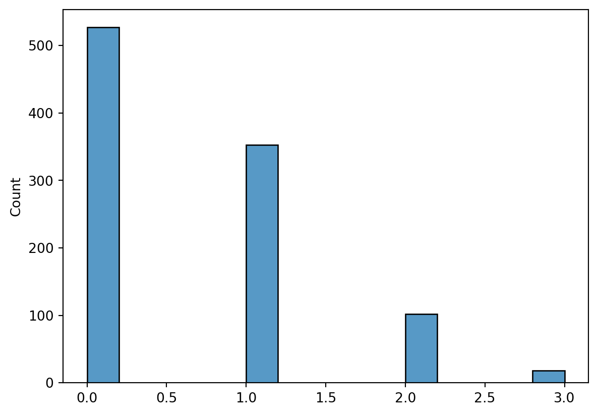

Negative Binomial

# this makes sense
v_negative_binomial = rng.negative_binomial(n = 1, p = 0.25, size = n)
sns.histplot(v_negative_binomial)

<AxesSubplot: ylabel='Count'>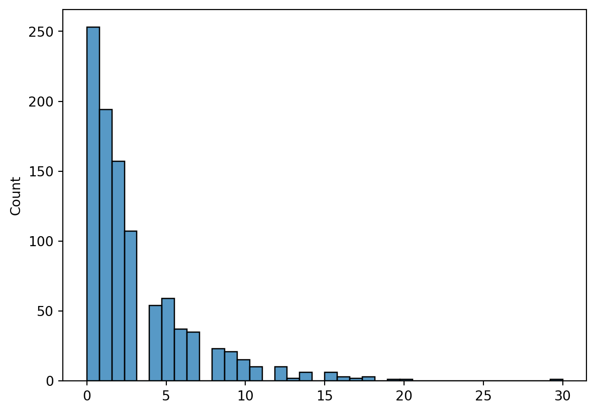

Modeling

Linear Regression

Another routine thing that will come up a lot is linear regression. It’s not as obvious as R, but it’s pretty straight-forward.

# you can use formula is you use smf 
linear_model = smf.ols(formula = 'wt ~ disp + mpg', data = df).fit()

We can get the results using sume summary() method, and it will look pretty familiar to R users.

linear_model.summary()

OLS Regression Results
Dep. Variable:	wt	R-squared:	0.836
Model:	OLS	Adj. R-squared:	0.824
Method:	Least Squares	F-statistic:	73.65
Date:	Fri, 27 Jan 2023	Prob (F-statistic):	4.31e-12
Time:	10:21:49	Log-Likelihood:	-15.323
No. Observations:	32	AIC:	36.65
Df Residuals:	29	BIC:	41.04
Df Model:	2
Covariance Type:	nonrobust

	coef	std err	t	P>\|t\|	[0.025	0.975]
Intercept	3.5627	0.699	5.094	0.000	2.132	4.993
disp	0.0043	0.001	3.818	0.001	0.002	0.007
mpg	-0.0663	0.023	-2.878	0.007	-0.113	-0.019

Omnibus:	0.431	Durbin-Watson:	1.028
Prob(Omnibus):	0.806	Jarque-Bera (JB):	0.579
Skew:	0.187	Prob(JB):	0.749
Kurtosis:	2.458	Cond. No.	2.52e+03

Notes:
[1] Standard Errors assume that the covariance matrix of the errors is correctly specified.
[2] The condition number is large, 2.52e+03. This might indicate that there are
strong multicollinearity or other numerical problems.

Logistic Regression

The next logical step is logistic regression. No surprises here.

# fit the model
logistic_model = smf.glm("am ~ wt + mpg", data = df,
  family = sm.families.Binomial()).fit()

logistic_model.summary()

Generalized Linear Model Regression Results
Dep. Variable:	am	No. Observations:	32
Model:	GLM	Df Residuals:	29
Model Family:	Binomial	Df Model:	2
Link Function:	Logit	Scale:	1.0000
Method:	IRLS	Log-Likelihood:	-8.5921
Date:	Fri, 27 Jan 2023	Deviance:	17.184
Time:	10:21:49	Pearson chi2:	32.7
No. Iterations:	7	Pseudo R-squ. (CS):	0.5569
Covariance Type:	nonrobust

	coef	std err	z	P>\|z\|	[0.025	0.975]
Intercept	25.8866	12.194	2.123	0.034	1.988	49.785
wt	-6.4162	2.547	-2.519	0.012	-11.407	-1.425
mpg	-0.3242	0.239	-1.354	0.176	-0.794	0.145

ANOVA

The next basic anaylsis I wanted to recreate was ANOVA. This is handled nicely by statsmodels, looking more or less like the previous models.

# fit the initial model
anova_model = smf.ols("cyl ~ mpg + disp", data = df).fit()

anova = sm.stats.anova_lm(anova_model)
anova

	df	sum_sq	mean_sq	F	PR(>F)
mpg	1.0	71.801048	71.801048	132.393794	2.496891e-12
disp	1.0	11.346399	11.346399	20.921600	8.274021e-05
Residual	29.0	15.727553	0.542329	NaN	NaN

Tukey Test

After an ANOVA, some sort of post-hoc test is usually preformed. This isn’t as obvious as the ones above, requiring us to specify monovariate vectors instead of using a formla.

# specify the groups without the formual
tukey_results = sm.stats.multicomp.pairwise_tukeyhsd(endog = df["mpg"],
  groups = df["cyl"])

print(tukey_results)

 Multiple Comparison of Means - Tukey HSD, FWER=0.05 
=====================================================
group1 group2 meandiff p-adj   lower    upper  reject
-----------------------------------------------------
     4      6  -6.9208 0.0003 -10.7693 -3.0722   True
     4      8 -11.5636    0.0 -14.7708 -8.3565   True
     6      8  -4.6429 0.0112  -8.3276 -0.9581   True
-----------------------------------------------------